python实现感知机模型python深度学习-

这篇文章通过对花鸢尾属植物进行分类，来学习如何利用实际数据构建一个感知机模型，（文末附GD和SGD参数更新手推公式）。

目录

一、数据集

二、需要导入的库

三、读取数据集

四、数据散点图可视化

五、利用感知机模型进行线性分类 

六、不同学习率损失可视化对比

七、归一化后分类

八、随机梯度下降

九、完整的代码

 十、公式推导：

一、数据集

Iris数据集是常用的分类实验数据集，由Fisher, 1936收集整理。Iris也称鸢尾花卉数据集，是一类多重变量分析的数据集。数据集包含150个数据样本，分为3类，每类50个数据，每个数据包含4个属性。可通过花萼长度，花萼宽度，花瓣长度，花瓣宽度4个属性预测鸢尾花卉属于（Setosa，Versicolour，Virginica）三个种类中的哪一类。

iris以鸢尾花的特征作为数据来源，常用在分类操作中。该数据集由3种不同类型的鸢尾花的各50个样本数据构成。其中的一个种类与另外两个种类是线性可分离的，后两个种类是非线性可分离的。

该数据集包含了4个属性：

& Sepal.Length（花萼长度），单位是cm;

& Sepal.Width（花萼宽度），单位是cm;

& Petal.Length（花瓣长度），单位是cm;

& Petal.Width（花瓣宽度），单位是cm;

种类：Iris Setosa（山鸢尾）、Iris Versicolour（杂色鸢尾），以及Iris Virginica（维吉尼亚鸢尾）。

二、需要导入的库

 import pandas as pd import matplotlib.pyplot as plt import numpy as np  from matplotlib.colors import ListedColormap #from sklearn.linear_model import Perceptron import Perceptron as perceptron_class

三、读取数据集

 df = pd.read_csv('https://archive.ics.uci.edu/ml/machine-learning-databases/iris/iris.data', header=None) df.tail() #抽取出前100条样本，这正好是Setosa和Versicolor对应的样本，我们将Versicolor对应的数据作为类别1，Setosa对应的作为-1。 # 对于特征，我们抽取出sepal length和petal length两维度特征，然后用散点图对数据进行可视化 #We extract the first 100 class labels that correspond to 50 Iris-Setosa and 50 Iris-Versicolor flowers. y = df.iloc[0:100, 4].values print(y)  y = np.where(y == 'Iris-setosa', -1, 1)#满足条件(condition)，输出x，不满足输出y。 print(y)  X = df.iloc[0:100, [0, 2]].values print(X) print(X.shape,y.shape)#(100,2) (100,)

结果：

 ['Iris-setosa' 'Iris-setosa' 'Iris-setosa' 'Iris-setosa' 'Iris-setosa'  'Iris-setosa' 'Iris-setosa' 'Iris-setosa' 'Iris-setosa' 'Iris-setosa'  'Iris-setosa' 'Iris-setosa' 'Iris-setosa' 'Iris-setosa' 'Iris-setosa'  'Iris-setosa' 'Iris-setosa' 'Iris-setosa' 'Iris-setosa' 'Iris-setosa'  'Iris-setosa' 'Iris-setosa' 'Iris-setosa' 'Iris-setosa' 'Iris-setosa'  'Iris-setosa' 'Iris-setosa' 'Iris-setosa' 'Iris-setosa' 'Iris-setosa'  'Iris-setosa' 'Iris-setosa' 'Iris-setosa' 'Iris-setosa' 'Iris-setosa'  'Iris-setosa' 'Iris-setosa' 'Iris-setosa' 'Iris-setosa' 'Iris-setosa'  'Iris-setosa' 'Iris-setosa' 'Iris-setosa' 'Iris-setosa' 'Iris-setosa'  'Iris-setosa' 'Iris-setosa' 'Iris-setosa' 'Iris-setosa' 'Iris-setosa'  'Iris-versicolor' 'Iris-versicolor' 'Iris-versicolor' 'Iris-versicolor'  'Iris-versicolor' 'Iris-versicolor' 'Iris-versicolor' 'Iris-versicolor'  'Iris-versicolor' 'Iris-versicolor' 'Iris-versicolor' 'Iris-versicolor'  'Iris-versicolor' 'Iris-versicolor' 'Iris-versicolor' 'Iris-versicolor'  'Iris-versicolor' 'Iris-versicolor' 'Iris-versicolor' 'Iris-versicolor'  'Iris-versicolor' 'Iris-versicolor' 'Iris-versicolor' 'Iris-versicolor'  'Iris-versicolor' 'Iris-versicolor' 'Iris-versicolor' 'Iris-versicolor'  'Iris-versicolor' 'Iris-versicolor' 'Iris-versicolor' 'Iris-versicolor'  'Iris-versicolor' 'Iris-versicolor' 'Iris-versicolor' 'Iris-versicolor'  'Iris-versicolor' 'Iris-versicolor' 'Iris-versicolor' 'Iris-versicolor'  'Iris-versicolor' 'Iris-versicolor' 'Iris-versicolor' 'Iris-versicolor'  'Iris-versicolor' 'Iris-versicolor' 'Iris-versicolor' 'Iris-versicolor'  'Iris-versicolor' 'Iris-versicolor'] [-1 -1 -1 -1 -1 -1 -1 -1 -1 -1 -1 -1 -1 -1 -1 -1 -1 -1 -1 -1 -1 -1 -1 -1  -1 -1 -1 -1 -1 -1 -1 -1 -1 -1 -1 -1 -1 -1 -1 -1 -1 -1 -1 -1 -1 -1 -1 -1  -1 -1  1  1  1  1  1  1  1  1  1  1  1  1  1  1  1  1  1  1  1  1  1  1   1  1  1  1  1  1  1  1  1  1  1  1  1  1  1  1  1  1  1  1  1  1  1  1   1  1  1  1] [[5.1 1.4]  [4.9 1.4]  [4.7 1.3]  [4.6 1.5]  [5.  1.4]  [5.4 1.7]  [4.6 1.4]  [5.  1.5]  [4.4 1.4]  [4.9 1.5]  [5.4 1.5]  [4.8 1.6]  [4.8 1.4]  [4.3 1.1]  [5.8 1.2]  [5.7 1.5]  [5.4 1.3]  [5.1 1.4]  [5.7 1.7]  [5.1 1.5]  [5.4 1.7]  [5.1 1.5]  [4.6 1. ]  [5.1 1.7]  [4.8 1.9]  [5.  1.6]  [5.  1.6]  [5.2 1.5]  [5.2 1.4]  [4.7 1.6]  [4.8 1.6]  [5.4 1.5]  [5.2 1.5]  [5.5 1.4]  [4.9 1.5]  [5.  1.2]  [5.5 1.3]  [4.9 1.5]  [4.4 1.3]  [5.1 1.5]  [5.  1.3]  [4.5 1.3]  [4.4 1.3]  [5.  1.6]  [5.1 1.9]  [4.8 1.4]  [5.1 1.6]  [4.6 1.4]  [5.3 1.5]  [5.  1.4]  [7.  4.7]  [6.4 4.5]  [6.9 4.9]  [5.5 4. ]  [6.5 4.6]  [5.7 4.5]  [6.3 4.7]  [4.9 3.3]  [6.6 4.6]  [5.2 3.9]  [5.  3.5]  [5.9 4.2]  [6.  4. ]  [6.1 4.7]  [5.6 3.6]  [6.7 4.4]  [5.6 4.5]  [5.8 4.1]  [6.2 4.5]  [5.6 3.9]  [5.9 4.8]  [6.1 4. ]  [6.3 4.9]  [6.1 4.7]  [6.4 4.3]  [6.6 4.4]  [6.8 4.8]  [6.7 5. ]  [6.  4.5]  [5.7 3.5]  [5.5 3.8]  [5.5 3.7]  [5.8 3.9]  [6.  5.1]  [5.4 4.5]  [6.  4.5]  [6.7 4.7]  [6.3 4.4]  [5.6 4.1]  [5.5 4. ]  [5.5 4.4]  [6.1 4.6]  [5.8 4. ]  [5.  3.3]  [5.6 4.2]  [5.7 4.2]  [5.7 4.2]  [6.2 4.3]  [5.1 3. ]  [5.7 4.1]] (100, 2) (100,)

四、数据散点图可视化

  plt.scatter(X[:50, 0], X[:50, 1],color='red', marker='o', label='setosa') plt.scatter(X[50:100, 0], X[50:100, 1],color='blue', marker='x', label='versicolor') plt.xlabel('sepal length') plt.ylabel('petal length') plt.legend(loc='upper left') plt.show()

五、利用感知机模型进行线性分类 

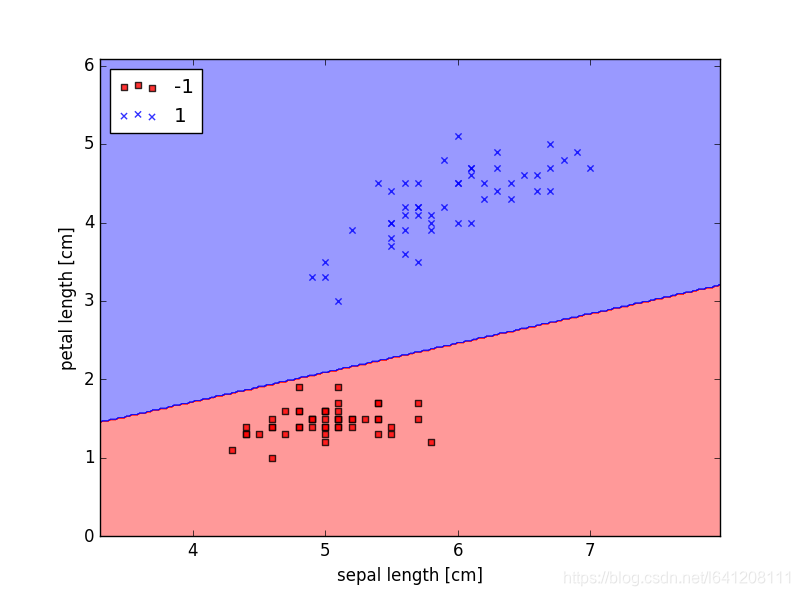
 #这里是对于感知机模型进行训练 ppn = perceptron_class.Perceptron(eta=0.1, n_iter=10) ppn.fit(X, y) #画出分界线  #To train our perceptron algorithm, plot the misclassification error plt.plot(range(1,len(ppn.errors_) + 1), ppn.errors_, marker='o') plt.xlabel('Epochs') plt.ylabel('Number of misclassifications') plt.show()  #Visualize the decision boundaries for 2D datasets def plot_decision_regions(X, y, classifier, resolution=0.02):     # setup marker generator and color map     markers = ('s', 'x', 'o', '^', 'v')     colors = ('red', 'blue', 'lightgreen', 'gray', 'cyan')     cmap = ListedColormap(colors[:len(np.unique(y))])     # plot the decision surface     x1_min, x1_max = X[:, 0].min() - 1, X[:, 0].max() + 1     x2_min, x2_max = X[:, 1].min() - 1, X[:, 1].max() + 1     xx1, xx2 = np.meshgrid(np.arange(x1_min, x1_max, resolution), np.arange(x2_min, x2_max, resolution))     Z = classifier.predict(np.array([xx1.ravel(), xx2.ravel()]).T)     Z = Z.reshape(xx1.shape)     print(xx1)     plt.contourf(xx1, xx2, Z, alpha=0.4, cmap=cmap)     plt.xlim(xx1.min(), xx1.max())     plt.ylim(xx2.min(), xx2.max())     # plot class samples     for idx, cl in enumerate(np.unique(y)):#除其中重复的元素，并按元素由大到小返回一个新的无元素重复的元组或者列表         plt.scatter(x=X[y == cl, 0], y=X[y == cl, 1],alpha=0.8, c=cmap(idx), marker=markers[idx],label=cl)   plot_decision_regions(X, y, classifier=ppn) plt.xlabel('sepal length [cm]') plt.ylabel('petal length [cm]') plt.legend(loc='upper left') plt.show()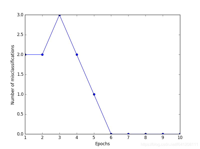

 分类误差： 

 分类结果：

六、不同学习率损失可视化对比

 #Adaptive linear neurons and the convergence of learning Implementing an Adaptive Linear Neuron in Python fig, ax = plt.subplots(nrows=1, ncols=2, figsize=(8,4)) ada1 = perceptron_class.AdalineGD(n_iter=10, eta=0.01).fit(X,y) ax[0].plot(range(1, len(ada1.cost_) + 1), np.log10(ada1.cost_), marker='o') ax[0].set_xlabel('Epochs') ax[0].set_ylabel('log(Sum-squared-error)') ax[0].set_title('Adaline - Learning rate 0.01') ada2 = perceptron_class.AdalineGD(n_iter=10, eta=0.0001).fit(X,y) ax[1].plot(range(1, len(ada2.cost_) + 1), ada2.cost_, marker='o') ax[1].set_xlabel('Epochs') ax[1].set_ylabel('Sum-squared-error') ax[1].set_title('Adaline - Learning rate 0.0001') plt.show()

七、归一化后分类

 #standardization  X_std = np.copy(X) X_std[:,0] = (X_std[:,0] - X_std[:,0].mean()) / X_std[:,0].std() X_std[:,1] = (X_std[:,1] - X_std[:,1].mean()) / X_std[:,1].std() ada = perceptron_class.AdalineGD(n_iter=15, eta=0.01) ada.fit(X_std, y) plot_decision_regions(X_std, y, classifier=ada) plt.title('Adaline - Gradient Descent') plt.xlabel('sepal length [standardized]') plt.ylabel('petal length [standardized]') plt.legend(loc='upper left') # plt.show() plt.plot(range(1, len(ada.cost_) + 1), ada.cost_, marker='o') plt.xlabel('Epochs') plt.ylabel('Sum-squared-error') plt.show()

八、随机梯度下降

 #Large scale machine learning and stochastic gradient descent ada = perceptron_class.AdalineSGD(n_iter=15, eta=0.01, random_state=1) ada.fit(X_std, y) plot_decision_regions(X_std, y, classifier=ada) plt.title('Adaline - Stochastic Gradient Descent') plt.xlabel('sepal length [standardized]') plt.ylabel('petal length [standardized]') plt.legend(loc='upper left') plt.show() plt.plot(range(1, len(ada.cost_) + 1), ada.cost_, marker='o') plt.xlabel('Epochs') plt.ylabel('Average Cost') plt.show()

九、完整的代码

 import pandas as pd import matplotlib.pyplot as plt import numpy as np  from matplotlib.colors import ListedColormap #from sklearn.linear_model import Perceptron import Perceptron as perceptron_class   df = pd.read_csv('https://archive.ics.uci.edu/ml/machine-learning-databases/iris/iris.data', header=None) df.tail() #抽取出前100条样本，这正好是Setosa和Versicolor对应的样本，我们将Versicolor对应的数据作为类别1，Setosa对应的作为-1。 # 对于特征，我们抽取出sepal length和petal length两维度特征，然后用散点图对数据进行可视化 #We extract the first 100 class labels that correspond to 50 Iris-Setosa and 50 Iris-Versicolor flowers. y = df.iloc[0:100, 4].values print(y)  y = np.where(y == 'Iris-setosa', -1, 1)#满足条件(condition)，输出x，不满足输出y。 print(y)  X = df.iloc[0:100, [0, 2]].values print(X) print(X.shape,y.shape)#(100,2) (100,)  plt.scatter(X[:50, 0], X[:50, 1],color='red', marker='o', label='setosa') plt.scatter(X[50:100, 0], X[50:100, 1],color='blue', marker='x', label='versicolor') plt.xlabel('sepal length') plt.ylabel('petal length') plt.legend(loc='upper left') plt.show()  #这里是对于感知机模型进行训练 ppn = perceptron_class.Perceptron(eta=0.1, n_iter=10) ppn.fit(X, y) #画出分界线  #To train our perceptron algorithm, plot the misclassification error plt.plot(range(1,len(ppn.errors_) + 1), ppn.errors_, marker='o') plt.xlabel('Epochs') plt.ylabel('Number of misclassifications') plt.show()  #Visualize the decision boundaries for 2D datasets def plot_decision_regions(X, y, classifier, resolution=0.02):     # setup marker generator and color map     markers = ('s', 'x', 'o', '^', 'v')     colors = ('red', 'blue', 'lightgreen', 'gray', 'cyan')     cmap = ListedColormap(colors[:len(np.unique(y))])     # plot the decision surface     x1_min, x1_max = X[:, 0].min() - 1, X[:, 0].max() + 1     x2_min, x2_max = X[:, 1].min() - 1, X[:, 1].max() + 1     xx1, xx2 = np.meshgrid(np.arange(x1_min, x1_max, resolution), np.arange(x2_min, x2_max, resolution))     Z = classifier.predict(np.array([xx1.ravel(), xx2.ravel()]).T)     Z = Z.reshape(xx1.shape)     print(xx1)     plt.contourf(xx1, xx2, Z, alpha=0.4, cmap=cmap)     plt.xlim(xx1.min(), xx1.max())     plt.ylim(xx2.min(), xx2.max())     # plot class samples     for idx, cl in enumerate(np.unique(y)):#除其中重复的元素，并按元素由大到小返回一个新的无元素重复的元组或者列表         plt.scatter(x=X[y == cl, 0], y=X[y == cl, 1],alpha=0.8, c=cmap(idx), marker=markers[idx],label=cl)   plot_decision_regions(X, y, classifier=ppn) plt.xlabel('sepal length [cm]') plt.ylabel('petal length [cm]') plt.legend(loc='upper left') plt.show()   #Adaptive linear neurons and the convergence of learning Implementing an Adaptive Linear Neuron in Python fig, ax = plt.subplots(nrows=1, ncols=2, figsize=(8,4)) ada1 = perceptron_class.AdalineGD(n_iter=10, eta=0.01).fit(X,y) ax[0].plot(range(1, len(ada1.cost_) + 1), np.log10(ada1.cost_), marker='o') ax[0].set_xlabel('Epochs') ax[0].set_ylabel('log(Sum-squared-error)') ax[0].set_title('Adaline - Learning rate 0.01') ada2 = perceptron_class.AdalineGD(n_iter=10, eta=0.0001).fit(X,y) ax[1].plot(range(1, len(ada2.cost_) + 1), ada2.cost_, marker='o') ax[1].set_xlabel('Epochs') ax[1].set_ylabel('Sum-squared-error') ax[1].set_title('Adaline - Learning rate 0.0001') plt.show()  #standardization  X_std = np.copy(X) X_std[:,0] = (X_std[:,0] - X_std[:,0].mean()) / X_std[:,0].std() X_std[:,1] = (X_std[:,1] - X_std[:,1].mean()) / X_std[:,1].std() ada = perceptron_class.AdalineGD(n_iter=15, eta=0.01) ada.fit(X_std, y) plot_decision_regions(X_std, y, classifier=ada) plt.title('Adaline - Gradient Descent') plt.xlabel('sepal length [standardized]') plt.ylabel('petal length [standardized]') plt.legend(loc='upper left') # plt.show() plt.plot(range(1, len(ada.cost_) + 1), ada.cost_, marker='o') plt.xlabel('Epochs') plt.ylabel('Sum-squared-error') plt.show()  #Large scale machine learning and stochastic gradient descent ada = perceptron_class.AdalineSGD(n_iter=15, eta=0.01, random_state=1) ada.fit(X_std, y) plot_decision_regions(X_std, y, classifier=ada) plt.title('Adaline - Stochastic Gradient Descent') plt.xlabel('sepal length [standardized]') plt.ylabel('petal length [standardized]') plt.legend(loc='upper left') plt.show() plt.plot(range(1, len(ada.cost_) + 1), ada.cost_, marker='o') plt.xlabel('Epochs') plt.ylabel('Average Cost') plt.show()

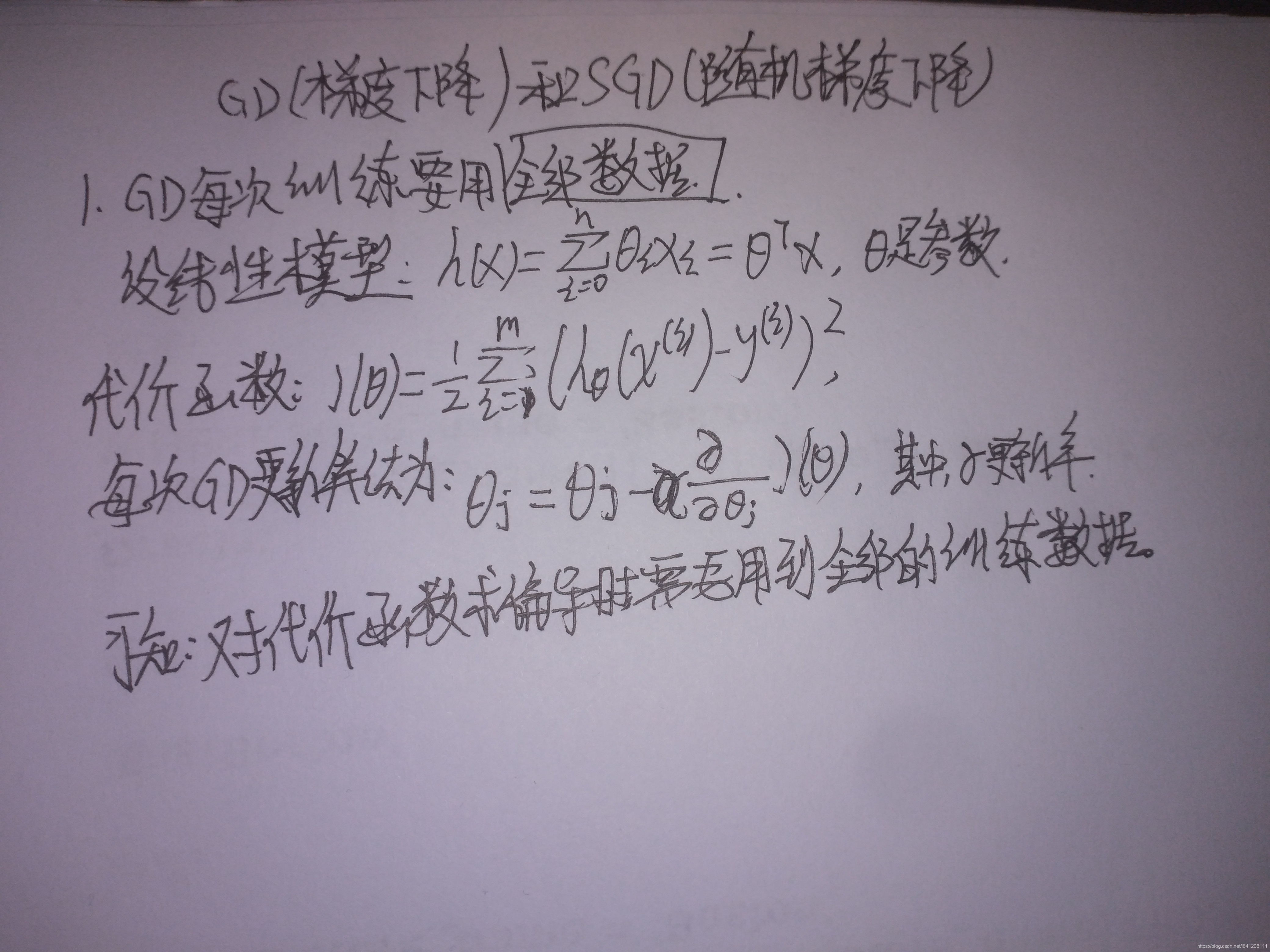
 import numpy as np from numpy.random import seed class Perceptron(object):     """Perceptron classifier.     Parameters     ------------     eta : float         Learning rate (between 0.0 and 1.0)     n_iter : int         Passes over the training dataset.     Attributes     -----------     w_ : 1d-array         Weights after fitting.     errors_ : list         Number of misclassifications (updates) in each epoch.     """     def __init__(self, eta=0.01, n_iter=10):         self.eta = eta         self.n_iter = n_iter      def fit(self, X, y):         """Fit training data.          Parameters         ----------         X : {array-like}, shape = [n_samples, n_features]             Training vectors, where n_samples is the number of samples and             n_features is the number of features.         y : array-like, shape = [n_samples]             Target values.          Returns         -------         self : object          """         self.w_ = np.zeros(1 + X.shape[1])         self.errors_ = []          for _ in range(self.n_iter):             errors = 0             for xi, target in zip(X, y):                 update = self.eta*(target - self.predict(xi))                 self.w_[1:] += update*xi                 self.w_[0] += update                 errors += int(update != 0.0)             self.errors_.append(errors)         return self      def net_input(self, X):         """Calculate net input"""         return np.dot(X, self.w_[1:]) + self.w_[0]      def predict(self, X):         """Return class label after unit step"""         return np.where(self.net_input(X) >= 0.0, 1, -1)   class AdalineGD(object):     """ADAptive LInear NEuron classifier.      Parameters     -------------     eta : float         Learning rate (between 0.0 and 1.0)     n_iter : int         Passes over the training dataset.      Attributes     -------------     w_ : 1d-array         Weights after fitting.     errors_ : list         Number of misclassifications in every epoch.      """     def __init__(self, eta=0.01, n_iter=50):         self.eta = eta         self.n_iter = n_iter      def fit(self, X, y):         """ Fit training data.          Parameters         ------------         X : {array-like5}, shape = [n_samples, n_features]             Training vectors,             where n_samples is the number of samples and             n_features is the number of features.         y　: array-like, shape = [n_samples]             Target values.          Returns         ------------         self : object           """         self.w_ = np.zeros(1 + X.shape[1])         self.cost_ = []          for i in range(self.n_iter):             output = self.net_input(X)             errors = (y - output)             self.w_[1:] += self.eta * X.T.dot(errors)             self.w_[0] += self.eta * errors.sum()             cost = (errors**2).sum() / 2.0             self.cost_.append(cost)         return self      def net_input(self, X):         """Calculate net input"""         return np.dot(X, self.w_[1:]) + self.w_[0]      def activation(self, X):         """Compute linear activation"""         return self.net_input(X)      def predict(self, X):         """Return class label after unit step"""         return np.where(self.activation(X) >= 0.0, 1, -1)  class AdalineSGD(object):     """ADAptive LInear NEuron classifier.      Parameters     ------------     eta : float         Learning rate (between 0.0 and 1.0)     n_iter : int         Passes over the training dataset.      Attributes     ------------     w_ : 1d-array         Weights after fitting.     cost_ : list         Number of misclassifications in every epoch.     shuffle : bool (default: True)         Shuffles training data every epoch         if True to prevent cycles.     random_state : int (default: None)         Set random state for shuffling         and initializing the weights.     """     def __init__(self, eta=0.01, n_iter=10, shuffle=True, random_state=None):         self.eta = eta         self.n_iter = n_iter         self.w_initialized = False         self.shuffle = shuffle         if random_state:             seed(random_state)      def fit(self, X, y):         """Fit training data.          Parameters         ------------         X : {array-like}, shape = [n_samples, n_features]             Training vector, where n_samples             is the number of samples and             n_features is the number of features.         y: arrary-like, shape = [n_samples]             Target values.          Returns         ------------         self : object          """         self._initialize_weights(X.shape[1])         self.cost_ = []         for i in range(self.n_iter):             if self.shuffle:                 X, y = self._shuffle(X, y)             cost = []             for xi, target in zip(X, y):                 cost.append(self._update_weights(xi, target))             avg_cost = sum(cost)/len(y)             self.cost_.append(avg_cost)         return self      def partial_fit(self, X, y):         """Fit training data without reinitializing the weights"""         if not self.w_initialized:             self._initialize_weights(X.shape[1])         if y.ravel().shape[0] > 1:             for xi, target in zip(X, y):                 self._update_weights(xi, target)         else:             self._update_weights(X, y)         return self      def _shuffle(self, X, y):         """Shuffle training data"""         r = np.random.permutation(len(y))         return X[r], y[r]      def _initialize_weights(self, m):         """Initialize weighs to zeros"""         self.w_ = np.zeros(1+m)         self.w_initialized = True      def _update_weights(self, xi, target):         """Apply Adaline learning rule to update the weights"""         output = self.net_input(xi)         error = (target - output)         self.w_[1:] += self.eta*xi.dot(error)         self.w_[0] += self.eta*error         cost = 0.5 * error**2         return cost      def net_input(self, X):         """Calculate net input"""         return np.dot(X, self.w_[1:]) + self.w_[0]      def activation(self, X):         """Compute linear activation"""         return self.net_input(X)      def predict(self, X):         """Return class label after unit step"""         return np.where(self.activation(X) >= 0.0, 1, -1)

 十、公式推导：