小黄人番外短片合集 — 第12集【Binky Nelson Unpacified 不消停的宾齐·尼尔森】 Matplotlib 系列文章(持续更新中): 直方图:直方图(Histogram)又称质量分布图,是一种统计报告图,由一系列高度不等的纵向条纹或线段表示数据分布的情况。一般用于描述连续型数据的分布关系,用横轴表示数据类型,纵轴表示分布情况。直方图是用面积表示各组频数的多少,矩形的高度表示每一组的频数或频率,宽度则表示各组的组距,因此其高度与宽度均有意义。其次,由于分组数据具有连续性,直方图的各矩形通常是连续排列。 柱状图:柱状图(bar chart)又称条图、长条图、柱状统计图、条状图、棒形图,是一种以长方形的长度为变量的统计图表。一般用于描述离散型分类数据的对比,长条图用来比较两个或以上的价值(不同时间或者不同条件),只有一个变量,通常利用于较小的数据集分析。柱状图亦可横向排列,或用多维方式表达。柱状图各矩形的宽度固定,矩形之间分开排列,会有间距。 条形图:通常情况下条形图 = 柱状图,也可以将横向排列的柱状图称为条形图。在本文中会将条形图视为后者。 基本语法: 基本参数: 其他参数: 参数 基本语法: 基本参数: 其他参数: 首先定义一个列表,其中的元素是与每个值对应的标准差, 在绘制多序列的柱状图时,只需要多次调用 所谓堆积图,就是将多序列数据堆积到一个矩形上显示,在柱状图中要实现堆积图,只需要改变 利用 基本语法: 其他参数: 与柱状图一样,首先定义一个列表,其中的元素是与每个值对应的标准差, 与多序列柱状图类似,在绘制多序列的条形图时,只需要多次调用 堆积图就是将多序列数据堆积到一个矩形上显示,和堆积的柱状图类似,在条形图中要实现堆积图,只需要改变 利用
文章目录
这里是一段防爬虫文本,请读者忽略。 本文原创首发于 ImapBox,作者 TRHX。 博客首页:https://itrhx.blog.csdn.net/ 本文链接:https://itrhx.blog.csdn.net/article/details/105952856
【1×00】直方图 / 柱状图 / 条形图的区别

【2×00】直方图的绘制
【2×01】函数介绍 matplotlib.pyplot.hist()
matplotlib.pyplot.hist() 函数用于绘制直方图。matplotlib.pyplot.hist(x[, bins=None, range=None, density=False, bottom=None, histtype='bar', align='mid', orientation='vertical', rwidth=None, log=False, color=None, label=None, stacked=False, **kwargs])
参数
描述
x
数据集,数组或数组序列
bins
统计的分布区间、条形数,可以是整数、序列或字符串,默认
rcParams["hist.bins"] =10
如果 bins 是整数,则定义的是等宽的矩形的个数
如果 bins 是序列,则定义的是每个矩形的区间,如:bins = [1, 2, 3, 4],则矩形分布区间为 [1,2)、[2,3)、[3,4]
如果 bins 是字符串,则它应该是 numpy.histogram_bin_edges 所支持的策略之一
range
矩形分布的区间,在没有指定 bins 生效,元组类型
density
是否显示频率统计结果,
频率统计结果=区间数目/(总数*区间宽度)
bottom
y 轴的起始位置,默认为 0
histtype
矩形的样式,有四种类型可选:
'bar':默认值,传统的条形直方图,如果给出多个数据,则条形图并排排列'barstacked':当数据为 1 个时,和 bar 结果一样,当数据为多个时,则进行垂直堆叠'step':未填充的线条形式;'stepfilled':填充的线条形式,效果与 bar 差不多
align
矩形的中心位于 bins(x 轴) 的位置,
'left':左;'mid':中;'right':右
orientation
矩形的方向,
vertical:垂直;horizontal:水平
rwidth
矩形的相对宽度,如果未指定,则自动计算宽度
log
y 坐标轴是否以指数刻度显示
color
矩形的颜色,默认蓝色,与 facecolor 作用相同,指定一个即可,如果两者都指定,则取 facecolor 的值
label
数据的标签,展示图例时使用
stacked
是否为堆积状图(当两个数据相似时,堆积在一起就会把第一个数据的显示相对缩小一点)
参数
描述
facecolor
标量或数组类型,每个矩形的颜色,与 color 作用相同,指定一个即可,如果两者都指定,则取 facecolor 的值
edgecolor
标量或数组类型,直方图边缘线的颜色
linewidth
标量或数组类型,直方图边缘线的宽度,如果为 0,则不绘制边
alpha
float 类型,矩形透明度
label
图例中显示的标签
linestyle / ls
线条样式,此处指矩形边缘线条样式
'-' or 'solid', '--' or 'dashed', '-.' or 'dashdot' or ':' or 'dotted', 'none' or ' ' or ''
linewidth / lw
线条宽度,此处指矩形边缘线的宽度,float 类型,默认 0.8
hatch
矩形的填充图案,可以是组合形式,如果有相同的图案,则会增加填充的密度
取值可以是:'/', '', '|', '-', '+', 'x', 'o', 'O', '.', '*'【2×02】简单直方图示例
import numpy as np import matplotlib.pyplot as plt plt.rcParams['font.sans-serif'] = ['Microsoft YaHei'] # 设置中文显示 x = np.random.randint(0, 101, 100) # 数据集 bins = np.arange(0, 101, 10) # 分布区间 [0,10)、[10,20)...[90,100] plt.hist(x, bins=bins, linewidth=0.5, edgecolor='k') # 边缘线宽0.5,颜色为黑色 plt.xlim(0, 100) # x 轴刻度范围 plt.title('简单直方图示例') # 标题 plt.xlabel('x axis label') # x 轴标签 plt.ylabel('y axis label') # y 轴标签 plt.show() 
【2×03】堆积的直方图
stacked 决定了将两份数据进行堆积显示。注意,有可能两个数据相似(y 轴的值相似),但是堆积在一起的时候,会把第一个数据的显示相对缩小一点。import matplotlib.pyplot as plt import numpy as np plt.rcParams['font.sans-serif'] = ['Microsoft YaHei'] hist1 = np.random.randint(0, 100, 100) hist2 = np.random.randint(0, 100, 100) x = [hist1, hist2] colors = ['orchid', 'deepskyblue'] labels = ['hist1', 'hist2'] bins = range(0, 101, 10) # 绘制两份数据的直方图,数据集等其他参数可以使用列表形式传递,也可以使用两次 hist 函数单独传递 plt.hist(x, bins=bins, color=colors, stacked=True, label=labels) plt.title('堆积的直方图示例') plt.xlabel('x axis label') plt.ylabel('y axis label') plt.legend(loc="upper left") plt.show() 
【2×04】填充其他样式
hatch 参数可以让直方图的矩形填充其他样式,可选值有:'/', '', '|', '-', '+', 'x', 'o', 'O', '.', '*'。可以是不同图案的组合形式,如果有相同的图案,则会增加填充的密度。import numpy as np import matplotlib.pyplot as plt plt.rcParams['font.sans-serif'] = ['Microsoft YaHei'] # 设置中文显示 x = np.random.randint(0, 101, 100) # 数据集 bins = np.arange(0, 101, 10) # 分布区间 [0,10)、[10,20)...[90,100] # 矩形颜色为白色,使用 / 填充,边缘线宽0.5,颜色为黑色 plt.hist(x, bins=bins, color='w', hatch='///', linewidth=0.5, edgecolor='k') plt.xlim(0, 100) # x 轴刻度范围 plt.title('直方图图案填充示例') # 标题 plt.xlabel('x axis label') # x 轴标签 plt.ylabel('y axis label') # y 轴标签 plt.show() 
【3×00】柱状图的绘制
【3×01】函数介绍 matplotlib.pyplot.bar()
matplotlib.pyplot.bar() 函数用于绘制柱状图。matplotlib.pyplot.bar(x, height[, width=0.8, bottom=None, align='center', **kwargs])
参数
描述
x
标量序列,每个矩形对应的 x 轴刻度
height
标量或标量序列,每个矩形对应的高度,即 y 轴刻度
width
标量或数组类型,每个矩形的宽度,默认为 0.8
bottom
标量或数组类型,y 轴的起始位置,默认为 0
align
矩形与 x 轴刻度对齐的位置,
'center':中;'edge':左边缘
参数
描述
color
标量或数组类型,每个矩形的颜色,与 facecolor 作用相同,指定一个即可,如果两者都指定,则取 facecolor 的值
edgecolor
标量或数组类型,柱状图边缘线的颜色
linewidth
标量或数组类型,柱状图边缘线的宽度,如果为0,则不绘制边
tick_label
标量或数组类型,柱状图 x 轴的刻度标签,默认使用数字标签
xerr / yerr
标量,指定对应标准差(添加误差线时会用到)
ecolor
标量或数组类型,误差线的线条颜色,默认值为 black
capsize
标量,误差线两头横线的宽度,默认为
rcParams["errorbar.capsize"] = 0.0
error_kw
字典类型,可以此字典中定义 ecolor 和 capsize,比单独指定的优先级要高
log
bool 值,y 坐标轴是否以指数刻度显示
alpha
float 类型,矩形透明度
label
图例中显示的标签
linestyle / ls
线条样式,此处指矩形边缘线条样式
'-' or 'solid', '--' or 'dashed', '-.' or 'dashdot' or ':' or 'dotted', 'none' or ' ' or ''
linewidth / lw
线条宽度,此处指矩形边缘线的宽度,float 类型,默认 0.8
hatch
矩形的填充图案,可以是组合形式,如果有相同的图案,则会增加填充的密度
取值可以是:'/', '', '|', '-', '+', 'x', 'o', 'O', '.', '*'【3×02】简单柱状图示例
import matplotlib.pyplot as plt plt.rcParams['font.sans-serif'] = ['Microsoft YaHei'] x = [1, 2, 3, 4, 5] height = [5, 7, 4, 3, 1] # 设置 x 轴的标签,也可以用 plt.xticks 方法来设置 tick_label = ['A', 'B', 'C', 'D', 'E'] # 设置颜色序列 color = ['red', 'yellow', 'peru', 'orchid', 'deepskyblue'] # 绘制柱状图,边缘线宽度为1,颜色为黑色,样式为 -- plt.bar(x, height, tick_label=tick_label, color=color, edgecolor='k', linewidth=1, linestyle='--') plt.title('简单柱状图示例') plt.xlabel('x axis label') plt.ylabel('y axis label') plt.show() 
【3×03】添加与标准差的误差线
ecolor 和 capsize 参数分别指定误差线的颜色和两头横线的宽度。这两个参数可以通过 error_kw 字典形式组合起来。以字典形式的组合优先级别要比单独指定高。另外,柱状图指定标准差时要用 yerr,条形图(横向排列的柱状图)指定标准差时要用 xerr。import matplotlib.pyplot as plt plt.rcParams['font.sans-serif'] = ['Microsoft YaHei'] x = [1, 2, 3, 4, 5] height = [5, 7, 4, 3, 2] std = [0.5, 0.1, 1.2, 0.3, 1.0] # 标准差 tick_label = ['A', 'B', 'C', 'D', 'E'] # 设置 x 轴的标签,也可以用 plt.xticks 方法来设置 color = ['red', 'yellow', 'peru', 'orchid', 'deepskyblue'] # 设置颜色序列 plt.bar( x, height, tick_label=tick_label, color=color, yerr=std, # 指定对应标准差 # error_kw={ # 'ecolor': 'k', # 指定误差线的颜色 # 'capsize': 6 # 指定误差线两头横线的宽度 # }, ecolor='k', capsize=6, edgecolor='k', # 指定边缘线颜色 linewidth=1 # 指定边缘线宽度 ) plt.title('柱状图添加误差线示例') plt.xlabel('x axis label') plt.ylabel('y axis label') plt.show() 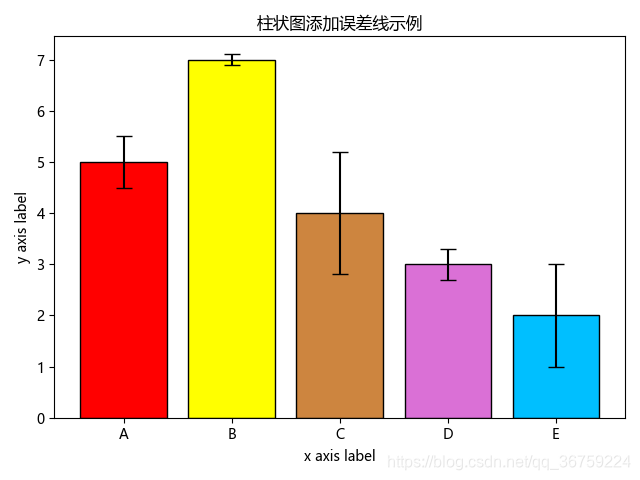
【3×04】多序列柱状图
matplotlib.pyplot.bar() 函数即可,指定一个较小的宽度值(偏移量),绘制不同数据时设置不同的 x 位置刻度即可。import numpy as np import matplotlib.pyplot as plt plt.rcParams['font.sans-serif'] = ['Microsoft YaHei'] x = np.arange(5) height1 = np.array([5, 7, 4, 3, 2]) height2 = np.array([2, 4, 6, 7, 3]) height3 = np.array([3, 1, 7, 5, 2]) # 设置宽度值(偏移量) width = 0.3 # 绘制不同数据时,x 轴依次增加一个偏移量 plt.bar(x, height1, width, label='bar1') plt.bar(x + width, height2, width, label='bar2') plt.bar(x + width * 2, height3, width, label='bar3') # 设置 x 轴刻度的标签 plt.xticks(x + width, ['A', 'B', 'C', 'D', 'E']) plt.title('多序列柱状图示例') plt.xlabel('x axis label') plt.ylabel('y axis label') plt.legend() plt.show() 
【3×05】堆积的柱状图
bottom 参数即可,bottom 参数用于设置 y 轴基线,即柱状图的底边在 y 轴上的起始刻度,第一条数据 data1 的基线可以设置为 0,即默认值,第二条数据 data2 的基线可以设置在 data1 的上方,即 bottom=data1,第三条数据 data3 的基线可以设置在 data1 + data2 的上方,即 bottom=data1+data2,以此类推。import numpy as np import matplotlib.pyplot as plt plt.rcParams['font.sans-serif'] = ['Microsoft YaHei'] x = np.arange(5) height1 = np.array([5, 7, 4, 3, 2]) height2 = np.array([2, 4, 6, 7, 3]) height3 = np.array([3, 1, 7, 5, 2]) plt.bar(x, height1, label='bar1') plt.bar(x, height2, label='bar2', bottom=height1) plt.bar(x, height3, label='bar3', bottom=(height2+height1)) plt.xticks(x, ['A', 'B', 'C', 'D', 'E']) plt.title('堆积的柱状图示例') plt.xlabel('x axis label') plt.ylabel('y axis label') plt.legend() plt.show() 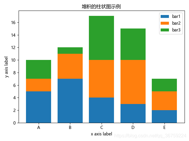
【3×06】填充其他样式
hatch 参数可以让柱状图的矩形填充其他样式,可选值有:'/', '', '|', '-', '+', 'x', 'o', 'O', '.', '*'。可以是不同图案的组合形式,如果有相同的图案,则会增加填充的密度。import numpy as np import matplotlib.pyplot as plt plt.rcParams['font.sans-serif'] = ['Microsoft YaHei'] x = np.arange(5) height1 = np.array([5, 7, 4, 3, 2]) height2 = np.array([2, 4, 6, 7, 3]) height3 = np.array([3, 1, 7, 5, 2]) plt.bar(x, height1, label='bar1', color='w', hatch='///') plt.bar(x, height2, label='bar2', bottom=height1, color='w', hatch='xxx') plt.bar(x, height3, label='bar3', bottom=(height2+height1), color='w', hatch='|||') plt.xticks(x, ['A', 'B', 'C', 'D', 'E']) plt.title('柱状图图案填充示例') plt.xlabel('x axis label') plt.ylabel('y axis label') plt.legend() plt.show() 
【3×07】添加文字描述
matplotlib.pyplot.text() 方法可以在柱状图每个矩形上方添加文字描述。具体参数解释可参考前面的文章:《Python 数据分析三剑客之 Matplotlib(二):文本描述 / 中文支持 / 画布 / 网格等基本图像属性》import numpy as np import matplotlib.pyplot as plt plt.rcParams['font.sans-serif'] = ['Microsoft YaHei'] x = np.arange(5) height1 = np.array([5, 7, 4, 3, 2]) height2 = np.array([2, 4, 6, 7, 3]) height3 = np.array([3, 1, 7, 5, 2]) width = 0.3 # 绘制不同数据时,x 轴依次增加一个偏移量 plt.bar(x, height1, width, label='bar1') plt.bar(x + width, height2, width, label='bar2') plt.bar(x + width * 2, height3, width, label='bar3') # 依次添加每条数据的标签 for a, b in zip(x, height1): plt.text(a, b, b, ha='center', va='bottom') for c, d in zip(x, height2): plt.text(c + width, d, d, ha='center', va='bottom') for e, f in zip(x, height3): plt.text(e + width * 2, f, f, ha='center', va='bottom') # 设置 x 轴刻度的标签 plt.xticks(x + width, ['A', 'B', 'C', 'D', 'E']) plt.title('柱状图添加文字描述示例') plt.xlabel('x axis label') plt.ylabel('y axis label') plt.legend() plt.show() 
【4×00】条形图的绘制
【4×01】函数介绍 matplotlib.pyplot.barh()
matplotlib.pyplot.barh() 函数用于绘制条形图(水平排列的柱状图)。matplotlib.pyplot.barh(y, width[, height=0.8, left=None, align='center', color, **kwargs])
参数
描述
y
标量或数组类型,每个矩形对应的 y 轴刻度
width
标量或数组类型,每个矩形的宽度,即 x 轴刻度
height
标量序列,每个矩形的高度,默认 0.8
left
标量序列,每个矩形的左侧 x 坐标的起始位置,默认值为 0
align
矩形的底边与 y 轴刻度对齐的位置,
'center':中;'edge':底边
参数
描述
color
标量或数组类型,每个矩形的颜色,与 facecolor 作用相同,指定一个即可,如果两者都指定,则取 facecolor 的值
edgecolor
标量或数组类型,条形图边缘线的颜色
linewidth
标量或数组类型,条形图边缘线的宽度,如果为0,则不绘制边
tick_label
标量或数组类型,条形图 y 轴的刻度标签,默认使用数字标签
xerr / yerr
标量,指定对应标准差(添加误差线时会用到)
ecolor
标量或数组类型,误差线的线条颜色,默认值为 black
capsize
标量,误差线两头横线的宽度,默认为
rcParams["errorbar.capsize"] = 0.0
error_kw
字典类型,可以此字典中定义 ecolor 和 capsize,比单独指定的优先级要高
log
bool 值,y 坐标轴是否以指数刻度显示
alpha
float 类型,矩形透明度
label
图例中显示的标签
linestyle / ls
线条样式,此处指矩形边缘线条样式
'-' or 'solid', '--' or 'dashed', '-.' or 'dashdot' or ':' or 'dotted', 'none' or ' ' or ''
linewidth / lw
线条宽度,此处指矩形边缘线的宽度,float 类型,默认 0.8
hatch
矩形的填充图案,可以是组合形式,如果有相同的图案,则会增加填充的密度
取值可以是:'/', '', '|', '-', '+', 'x', 'o', 'O', '.', '*'【4×02】简单条形图示例
import matplotlib.pyplot as plt plt.rcParams['font.sans-serif'] = ['Microsoft YaHei'] y = [1, 2, 3, 4, 5] width = [5, 7, 4, 3, 1] tick_label = ['A', 'B', 'C', 'D', 'E'] color = ['red', 'yellow', 'peru', 'orchid', 'deepskyblue'] plt.barh(y, width, tick_label=tick_label, color=color, edgecolor='k', linewidth=1, linestyle='--') plt.title('简单条形图示例') plt.xlabel('x axis label') plt.ylabel('y axis label') plt.show() 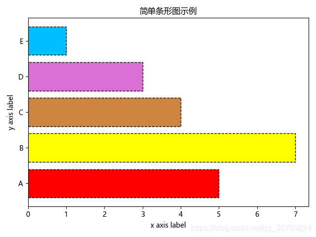
【4×03】添加与标准差的误差线
ecolor 和 capsize 参数分别指定误差线的颜色和两头横线的宽度。这两个参数可以通过 error_kw 字典形式组合起来。以字典形式的组合优先级别要比单独指定高。另外,柱状图指定标准差时要用 yerr,条形图(横向排列的柱状图)指定标准差时要用 xerr。import matplotlib.pyplot as plt plt.rcParams['font.sans-serif'] = ['Microsoft YaHei'] y = [1, 2, 3, 4, 5] width = [5, 7, 4, 3, 2] std = [0.5, 0.1, 1.2, 0.3, 1.0] # 标准差 tick_label = ['A', 'B', 'C', 'D', 'E'] # 设置 x 轴的标签,也可以用 plt.xticks 方法来设置 color = ['red', 'yellow', 'peru', 'orchid', 'deepskyblue'] # 颜色序列 plt.barh( y, width, tick_label=tick_label, color=color, xerr=std, # 指定对应标准差 # error_kw={ # 'ecolor': 'k', # 指定误差线的颜色 # 'capsize': 6 # 指定误差线两头横线的宽度 # }, ecolor='k', capsize=6, edgecolor='k', # 指定边缘线颜色 linewidth=1 # 指定边缘线宽度 ) plt.title('条形图添加误差线示例') plt.xlabel('x axis label') plt.ylabel('y axis label') plt.show() 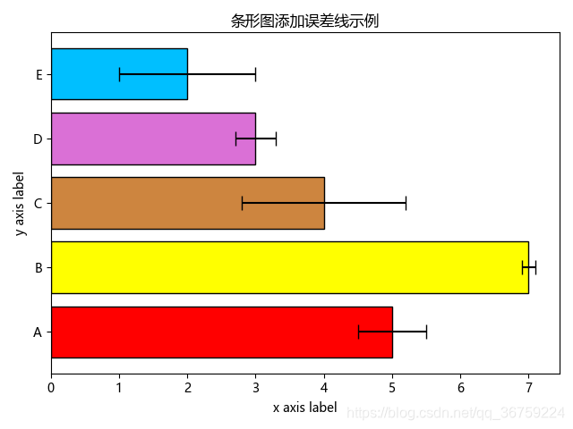
【4×04】多序列条形图
matplotlib.pyplot.barh() 函数即可,指定一个较小的高度值(偏移量),绘制不同数据时设置不同的 y 位置刻度即可。import numpy as np import matplotlib.pyplot as plt plt.rcParams['font.sans-serif'] = ['Microsoft YaHei'] y = np.arange(5) width1 = np.array([5, 7, 4, 3, 2]) width2 = np.array([2, 4, 6, 7, 3]) width3 = np.array([3, 1, 7, 5, 2]) # 设置高度值(偏移量) height = 0.3 # 绘制不同数据时,y 轴依次增加一个偏移量 plt.barh(y, width1, height, label='bar1') plt.barh(y + height, width2, height, label='bar2') plt.barh(y + height * 2, width3, height, label='bar3') # 设置 y 轴刻度的标签 plt.yticks(y + height, ['A', 'B', 'C', 'D', 'E']) plt.title('多序列条形图示例') plt.xlabel('x axis label') plt.ylabel('y axis label') plt.legend() plt.show() 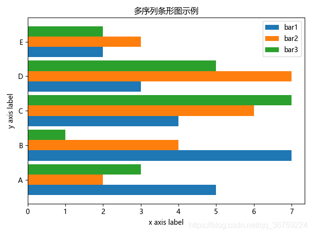
【4×05】堆积的条形图
left 参数即可,left 参数用于设置 x 轴基线,即柱状图的底边在 x 轴上的起始刻度,第一条数据 data1 的基线可以设置为 0,即默认值,第二条数据 data2 的基线可以设置在 data1 的上方,即 left=data1,第三条数据 data3 的基线可以设置在 data1 + data2 的上方,即 left=data1+data2,以此类推。import numpy as np import matplotlib.pyplot as plt plt.rcParams['font.sans-serif'] = ['Microsoft YaHei'] y = np.arange(5) width1 = np.array([5, 7, 4, 3, 2]) width2 = np.array([2, 4, 6, 7, 3]) width3 = np.array([3, 1, 7, 5, 2]) plt.barh(y, width1, label='bar1') plt.barh(y, width2, label='bar2', left=width1) plt.barh(y, width3, label='bar3', left=(width1+width2)) plt.yticks(y, ['A', 'B', 'C', 'D', 'E']) plt.title('堆积的条形图示例') plt.xlabel('x axis label') plt.ylabel('y axis label') plt.legend() plt.show() 
【4×06】填充其他样式
hatch 参数可以让柱状图的矩形填充其他样式,可选值有:'/', '', '|', '-', '+', 'x', 'o', 'O', '.', '*'。可以是不同图案的组合形式,如果有相同的图案,则会增加填充的密度。import numpy as np import matplotlib.pyplot as plt plt.rcParams['font.sans-serif'] = ['Microsoft YaHei'] y = np.arange(5) width1 = np.array([5, 7, 4, 3, 2]) width2 = np.array([2, 4, 6, 7, 3]) width3 = np.array([3, 1, 7, 5, 2]) plt.barh(y, width1, label='bar1', color='w', hatch='///') plt.barh(y, width2, label='bar2', left=width1, color='w', hatch='xxx') plt.barh(y, width3, label='bar3', left=(width1+width2), color='w', hatch='|||') plt.yticks(y, ['A', 'B', 'C', 'D', 'E']) plt.title('条形图图案填充示例') plt.xlabel('x axis label') plt.ylabel('y axis label') plt.legend() plt.show() 
【4×07】添加文字描述
matplotlib.pyplot.text() 方法可以在条形图每个矩形上方添加文字描述。具体参数解释可参考前面的文章:《Python 数据分析三剑客之 Matplotlib(二):文本描述 / 中文支持 / 画布 / 网格等基本图像属性》import numpy as np import matplotlib.pyplot as plt plt.rcParams['font.sans-serif'] = ['Microsoft YaHei'] y = np.arange(5) width1 = np.array([5, 7, 4, 3, 2]) width2 = np.array([2, 4, 6, 7, 3]) width3 = np.array([3, 1, 7, 5, 2]) height = 0.3 # 绘制不同数据时,y 轴依次增加一个偏移量 plt.barh(y, width1, height, label='bar1') plt.barh(y + height, width2, height, label='bar2') plt.barh(y + height * 2, width3, height, label='bar3') # 依次添加每条数据的标签 for a, b in zip(width1, y): plt.text(a, b-0.05, a) for c, d in zip(width2, y): plt.text(c, d+0.20, c) for e, f in zip(width3, y): plt.text(e, f+0.50, e) # 设置 y 轴刻度的标签 plt.yticks(y + height, ['A', 'B', 'C', 'D', 'E']) plt.title('条形图添加文字描述示例') plt.xlabel('x axis label') plt.ylabel('y axis label') plt.legend() plt.show() 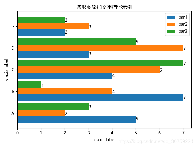
本网页所有视频内容由 imoviebox边看边下-网页视频下载, iurlBox网页地址收藏管理器 下载并得到。
ImovieBox网页视频下载器 下载地址: ImovieBox网页视频下载器-最新版本下载
本文章由: imapbox邮箱云存储,邮箱网盘,ImageBox 图片批量下载器,网页图片批量下载专家,网页图片批量下载器,获取到文章图片,imoviebox网页视频批量下载器,下载视频内容,为您提供.
阅读和此文章类似的: 全球云计算
 官方软件产品操作指南 (170)


 博客专家
博客专家 


 9756
9756