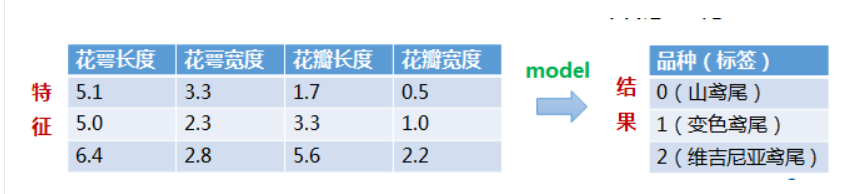
一个机器学习的小应用:鸢尾花分类 上面的代码就完成了数据集的准备 其中百分之70作为训练集 百分之30作为测试集 所以 上述代码 test_size=0.3 接下来便开始模型的训练! 模型训练完成后 就要开始对模型能力进行评估: 可以看见出现了如下输出结果: 最后成功绘图: 谢谢大家,期待下次更新
鸢尾花有很多种,我们今天具体分类三种:
1.山鸢尾:

维吉尼亚鸢尾:
变色鸢尾:
看的出来,每个都很beautiful😀,但又都不一样
然后本文数据集和部分代码来自百度飞桨平台:
https://aistudio.baidu.com/aistudio/projectdetail/449373?forkThirdPart=1
我们可以看到数据集是150行的5列的数据:
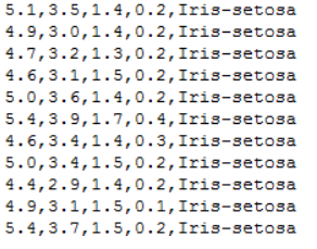
import numpy as np from matplotlib import colors from sklearn import svm from sklearn.svm import SVC from sklearn import model_selection import matplotlib.pyplot as plt import matplotlib as mpl #导入必要的库 #*************将字符串转为整型,便于数据加载*********************** def iris_type(s): it = {b'Iris-setosa':0, b'Iris-versicolor':1, b'Iris-virginica':2} return it[s] #将山鸢尾标为0 变色鸢尾花为1 维吉尼亚鸢尾花为2 #加载数据 data_path='/home/aistudio/data/data2301/iris.data' #数据文件的路径 data = np.loadtxt(data_path, #数据文件路径 dtype=float, #数据类型 delimiter=',', #数据分隔符 converters={4:iris_type}) #将第5列使用函数iris_type进行转换 第五列就是种类了 # print(data) #data为二维数组,data.shape=(150, 5) # print(data.shape) #数据分割 x, y = np.split(data, #要切分的数组 (4,), #沿轴切分的位置,第5列开始往后为y axis=1) #代表纵向分割,按列分割 x = x[:, 0:2] #在X中我们取前两列作为特征,为了后面的可视化。x[:,0:2]代表第一维(行)全取,第二维(列)取0~2 print(x) x_train,x_test,y_train,y_test=model_selection.train_test_split(x, #所要划分的样本特征集 y, #所要划分的样本结果 random_state=1, #随机数种子 test_size=0.3) #测试样本占比
下面就开始模型的搭建:
我们将使用SVM向量机来完成。

支持向量机(Support Vector Machine, SVM)是一类按监督学习(supervised learning)方式对数据进行二元分类的广义线性分类器(generalized linear classifier),其决策边界是对学习样本求解的最大边距超平面(maximum-margin hyperplane) [1-3] 。
SVM使用铰链损失函数(hinge loss)计算经验风险(empirical risk)并在求解系统中加入了正则化项以优化结构风险(structural risk),是一个具有稀疏性和稳健性的分类器 [2] 。SVM可以通过核方法(kernel method)进行非线性分类,是常见的核学习(kernel learning)方法之一 [4] 。
SVM被提出于1964年,在二十世纪90年代后得到快速发展并衍生出一系列改进和扩展算法,在人像识别、文本分类等模式识别(pattern recognition)问题中有得到应用 ——取值百度百科。#**********************SVM分类器构建************************* def classifier(): #clf = svm.SVC(C=0.8,kernel='rbf', gamma=50,decision_function_shape='ovr') clf = svm.SVC(C=0.5, #误差项惩罚系数,默认值是1 kernel='linear', #线性核 kenrel="rbf":高斯核 decision_function_shape='ovr') #决策函数 return clf # 2.定义模型:SVM模型定义 clf = classifier() #***********************训练模型***************************** def train(clf,x_train,y_train): clf.fit(x_train, #训练集特征向量 y_train.ravel()) #训练集目标值 # 3.训练SVM模型 train(clf,x_train,y_train) #**************并判断a b是否相等,计算acc的均值************* def show_accuracy(a, b, tip): acc = a.ravel() == b.ravel() print('%s Accuracy:%.3f' %(tip, np.mean(acc))) def print_accuracy(clf,x_train,y_train,x_test,y_test): #分别打印训练集和测试集的准确率 score(x_train,y_train):表示输出x_train,y_train在模型上的准确率 print('trianing prediction:%.3f' %(clf.score(x_train, y_train))) print('test data prediction:%.3f' %(clf.score(x_test, y_test))) #原始结果与预测结果进行对比 predict()表示对x_train样本进行预测,返回样本类别 show_accuracy(clf.predict(x_train), y_train, 'traing data') show_accuracy(clf.predict(x_test), y_test, 'testing data') #计算决策函数的值,表示x到各分割平面的距离 print('decision_function:n', clf.decision_function(x_train)) # 4.模型评估 print_accuracy(clf,x_train,y_train,x_test,y_test)

之后便将模型使用,同时做到数据可视化:def draw(clf, x): iris_feature = 'sepal length', 'sepal width', 'petal lenght', 'petal width' # 开始画图 x1_min, x1_max = x[:, 0].min(), x[:, 0].max() #第0列的范围 x2_min, x2_max = x[:, 1].min(), x[:, 1].max() #第1列的范围 x1, x2 = np.mgrid[x1_min:x1_max:200j, x2_min:x2_max:200j] #生成网格采样点 grid_test = np.stack((x1.flat, x2.flat), axis=1) #stack():沿着新的轴加入一系列数组 print('grid_test:n', grid_test) # 输出样本到决策面的距离 z = clf.decision_function(grid_test) print('the distance to decision plane:n', z) grid_hat = clf.predict(grid_test) # 预测分类值 得到【0,0.。。。2,2,2】 print('grid_hat:n', grid_hat) grid_hat = grid_hat.reshape(x1.shape) # reshape grid_hat和x1形状一致 #若3*3矩阵e,则e.shape()为3*3,表示3行3列 cm_light = mpl.colors.ListedColormap(['#A0FFA0', '#FFA0A0', '#A0A0FF']) cm_dark = mpl.colors.ListedColormap(['g', 'r', 'b']) plt.pcolormesh(x1, x2, grid_hat, cmap=cm_light) # pcolormesh(x,y,z,cmap)这里参数代入 # x1,x2,grid_hat,cmap=cm_light绘制的是背景。 plt.scatter(x[:, 0], x[:, 1], c=np.squeeze(y), edgecolor='k', s=50, cmap=cm_dark) # 样本点 plt.scatter(x_test[:, 0], x_test[:, 1], s=120, facecolor='none', zorder=10) # 测试点 plt.xlabel(iris_feature[0], fontsize=20) plt.ylabel(iris_feature[1], fontsize=20) plt.xlim(x1_min, x1_max) plt.ylim(x2_min, x2_max) plt.title('svm in iris data classification', fontsize=30) plt.grid() plt.show()

想对代码重复的建议登陆百度AI平台在线编辑。
数据集也可以在上面网址下载。
😀
本网页所有视频内容由 imoviebox边看边下-网页视频下载, iurlBox网页地址收藏管理器 下载并得到。
ImovieBox网页视频下载器 下载地址: ImovieBox网页视频下载器-最新版本下载
本文章由: imapbox邮箱云存储,邮箱网盘,ImageBox 图片批量下载器,网页图片批量下载专家,网页图片批量下载器,获取到文章图片,imoviebox网页视频批量下载器,下载视频内容,为您提供.
阅读和此文章类似的: 全球云计算
 官方软件产品操作指南 (170)


