机器学习之手写数字识别大作业报告人工智能阿坨的博客-

写在前面

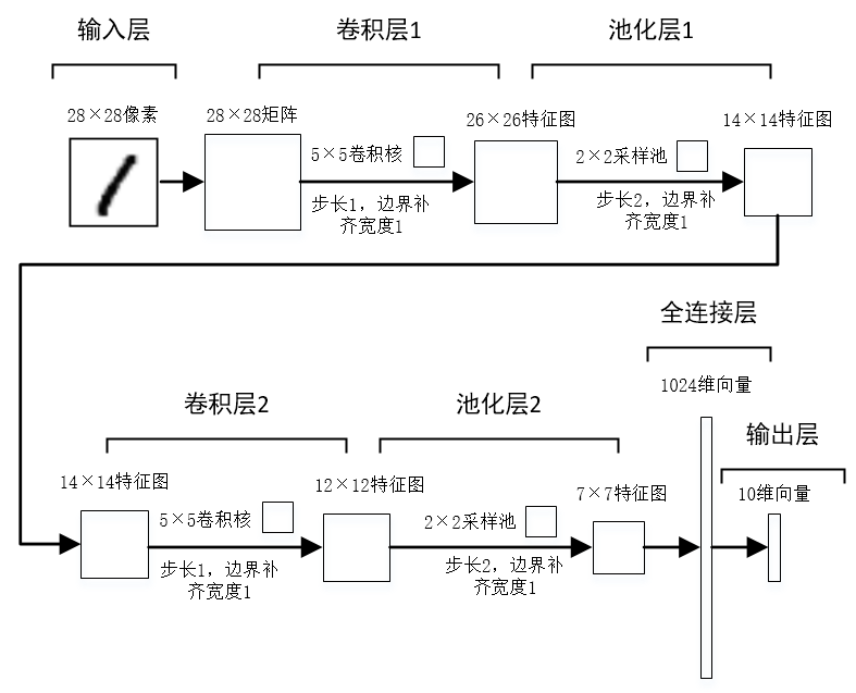
在选择特征的时候，曾纠结过是用颜色矩、像素值还是图片卷积过后的值作为特征，我选择了后者，因为个人觉得手写数字识别相对于水质颜色识别来说，更关注图片的二维结构信息，如果用颜色矩或者像素值作为特征，就把图片的二维结构信息拆散了，这对于模型训练来说，是得不偿失的。本次大作业步骤分为以下几步。

步骤一：图片尺寸归一化

经过观察，trainImages和testImages文件夹下的图片尺寸不一，在构建特征集之前需要把图片尺寸归一化。

在trainImages和testImages文件夹下，提取目录下所有图片,更改尺寸后再保存回trainImages，testImages目录中。

# test1.py from PIL import Image import os.path import glob def convertjpg(jpgfile,outdir,width=28,height=28):     img=Image.open(jpgfile) try:         new_img=img.resize((width,height),Image.BILINEAR)         new_img.save(os.path.join(outdir,os.path.basename(jpgfile))) except Exception as e: print(e) for jpgfile in glob.glob(r".trainImages*.png"):     convertjpg(jpgfile,r".trainImages") 

此时trainImages和testImages文件夹下已经经过图片尺寸归一化。

步骤二：把图片转为像素矩阵并获取图片标签

把每一张28 x 28的图片分别转为长度为784的向量，再合并成一个大的像素矩阵pixel_data，并获取图片标签，函数功能封装如下。

# test2.py from PIL import Image import numpy as np import re import os  path = r".trainImages" #获取训练集和测试集图片名称 def get_img_names(path=path):     file_names = os.listdir(path)     img_names = [] for i in file_names: if re.findall('^d_d+.png$', i) != []:             img_names.append(i) return img_names  #获取图片像素大矩阵，每一张图片占一行向量 def get_img_data(img_names):     pixel_data = [] for i in img_names:         img = Image.open(".\trainImages\" + i) #因为图片是黑白图像，我只取一个颜色通道的像素信息作为特征集         img_vector = np.array(img.split()[0]).reshape(1,784)[0]         pixel_data.append(img_vector) #像素数据归一化到0-1之间，便于模型训练     pixel_data = np.array(pixel_data) / 255 return pixel_data  #获取图片标签 def get_img_label(img_names):     n = len(img_names)     labels = np.zeros([n]) for i in range(len(img_names)):         labels[i] = img_names[i][0] return labels 

步骤三：随机从训练集中取batch_size个训练样本

现在调用步骤二的函数获得训练集和测试集的特征和标签，接下来需要做的是实现从训练集中随机取batch_size个训练样本，以便后期供给模型训练，功能函数封装在test3.py中，在模型训练中，可以调用test3.next_batch()获得训练样本和测试样本，并且在test3.py中我把图片标签转为独热编码的形式。

# test3.py # 随机取batch_size个训练样本 import numpy as np import pandas as pd from test2 import * #训练特征集 train_img_names = get_img_names() train_feature = get_img_data(train_img_names) #训练标签集，转为独热编码 train_labels = get_img_label(train_img_names) train_labels = np.array(pd.get_dummies(np.array(train_labels))) #测试集特征集 test_path = r".testImages" test_img_names = get_img_names(path=test_path) test_feature = get_img_data(test_img_names) #训练标签集，也转为独热编码 test_labels = get_img_label(test_img_names) test_labels = np.array(pd.get_dummies(np.array(test_labels))) #train_data训练集特征，train_target训练集对应的标签，batch_size def next_batch(batch_size,train_data = train_feature, train_target = train_labels): #打乱数据集     index = [ i for i in range(0,len(train_target)) ]     np.random.shuffle(index); #建立batch_data与batch_target的空列表     batch_data = [];     batch_target = []; #向空列表加入训练集及标签 for i in range(0,batch_size):         batch_data.append(train_data[index[i]]);         batch_target.append(train_target[index[i]])     batch_data = np.array(batch_data)     batch_target = np.array(batch_target) return batch_data, batch_target 

步骤四：构建模型

使用到的模型是卷积神经网络，卷积神经网络对比传统的BP神经网络而言，能够保留图片的二维结构信息，使用卷积神经网络来识别手写数字图片，是合适的。关于卷积神经网络的简单认识，个人有整理过一篇博客：一文简单介绍卷积神经网络（CNN）。

下面使用TensorFlow来构建卷积神经网络并进行模型训练和预测，具体的模型结构流程如下图。

使用到的TensorFlow代码有参考自TensorFlow官网：MNIST进阶 | TensorFlow，我的TensorFlow版本为1.14。

# model.py import tensorflow as tf import numpy as np import test3  #------------------------模型构建如下---------------------------- #定义会话 sess = tf.compat.v1.InteractiveSession() #占位符 x = tf.compat.v1.placeholder("float", shape=[None, 784]) y_ = tf.compat.v1.placeholder("float", shape=[None, 10]) #采用函数的形式定义权重 def weight_variable(shape):   initial = tf.random.truncated_normal(shape, stddev=0.1) return tf.Variable(initial) #采用函数的形式定义偏置量 def bias_variable(shape):   initial = tf.constant(0.1, shape=shape) return tf.Variable(initial) #定义卷积函数 def conv2d(x, w): return tf.nn.conv2d(x, w, strides=[1, 1, 1, 1], padding='SAME') #定义池化函数 def max_pool_2x2(x): return tf.nn.max_pool2d(x, ksize=[1, 2, 2, 1], strides=[1, 2, 2, 1], padding='SAME') #定义第一层卷积核filter和偏置量，偏置量的维度是32. W_conv1 = weight_variable([5, 5, 1, 32]) b_conv1 = bias_variable([32]) # 将输入tensor进行形状调整，调整成为一个28*28的图片 x_image = tf.reshape(x, [-1,28,28,1]) #进行第一层卷积操作，得到线性变化的结果再利用relu规则进行非线性映射，得到第一层卷积结果h_conv1。 h_conv1 = tf.nn.relu(conv2d(x_image, W_conv1) + b_conv1) #采用了最大池化方法，最终得出池化结果h_pool1 h_pool1 = max_pool_2x2(h_conv1) #定义第二层卷积核filter和偏置量，偏置量的维度是64. W_conv2 = weight_variable([5, 5, 32, 64]) b_conv2 = bias_variable([64]) # 第二层卷积和池化结果 h_conv2 = tf.nn.relu(conv2d(h_pool1, W_conv2) + b_conv2) h_pool2 = max_pool_2x2(h_conv2) #定义全连接层的权重和偏置量 W_fc1 = weight_variable([7 * 7 * 64, 1024]) b_fc1 = bias_variable([1024]) #将第二层池化后的数据调整为7×7×64的向量 #再与全连接层的权重进行矩阵相乘，然后进行非线性映射得到1024维的向量。 h_pool2_flat = tf.reshape(h_pool2, [-1, 7*7*64]) h_fc1 = tf.nn.relu(tf.matmul(h_pool2_flat, W_fc1) + b_fc1)  keep_prob = tf.compat.v1.placeholder("float") h_fc1_drop = tf.nn.dropout(h_fc1, keep_prob) #输出层的权重和偏置量 W_fc2 = weight_variable([1024, 10]) b_fc2 = bias_variable([10]) #添加softmax，得到输出结果 y_conv=tf.nn.softmax(tf.matmul(h_fc1_drop, W_fc2) + b_fc2) #损失函数 cross_entropy = -tf.reduce_sum(y_*tf.math.log(y_conv)) #梯度下降法 train_step = tf.compat.v1.train.AdamOptimizer(1e-4).minimize(cross_entropy) #模型精度 correct_prediction = tf.equal(tf.argmax(y_conv,1), tf.argmax(y_,1)) accuracy = tf.reduce_mean(tf.cast(correct_prediction, "float")) #--------------------------模型训练如下------------------------- # 先通过tf执行全局变量的初始化，然后启用session运行图。 sess.run(tf.compat.v1.global_variables_initializer()) for i in range(500):   batch = test3.next_batch(20)   batch_feature = batch[0]   batch_label = batch[1] if i % 100 == 0:     train_accuracy = accuracy.eval(feed_dict={x:batch_feature, y_: batch_label, keep_prob: 1.0}) print("第 %d 轮迭代, 手写数字识别训练集精度 %g"%(i, train_accuracy))   train_step.run(feed_dict={x: batch_feature, y_: batch_label, keep_prob: 0.5}) print("手写数字识别测试集精度 %g" % accuracy.eval(feed_dict={x: test3.test_feature, y_:test3.test_labels , keep_prob: 1.0})) 

执行500轮迭代，每轮随机喂20个样本。

运行结果

可以看到，模型在200轮迭代时候，模型在训练集上和测试集上的精度能达到100%，能取得这种精度的原因我觉得有：使用的卷积神经网络模型能很大限度地保留图片的二维信息，训练集和测试集的样本数据不多。